Monte Carlo Cost Estimates: Engineers Throwing Dice

Peter Prevos |
2059 words | 10 minutes
Share this content
Estimating the cost of a complex project is not a trivial task. Traditional cost estimates are full of assumptions about the future state of the market and the final deliverable. Monte Carlo cost estimates are a tool for better understanding your project's risks and enabling better cost control. Monte Carlo simulations are a technique to control your “known unknowns”.
Albert Einstein famously said that “God does not play dice”. While this might or might not be the case, engineers play dice and embrace the stochastic nature of reality to predict the future. Monte Carlo Simulations are a method for estimating the cost of your project across thousands of parallel universes to assess financial risk.
While I have a pet hate against using matrices to manage risk, Monte Carlo simulations are an analytical method for dealing with uncertainty and risk. This article explains the principles of Monte Carlo cost estimates and how to implement them in the R language for statistical computing.
You can download the code from GitHub in the case-studies folder.
The principles of cost estimates
The basic principle of cost estimation is deceptively simple. To estimate the cost for each item in a project, multiply the quantity of work $Q_i$ times the rate $R_i$ you will pay for each unit of work. Sum the cost of each item, and you have the total project cost $P$ for a project with $j$ items:
$$P = \sum_{i=1}^j Q_i R_i$$
The reality is, unfortunately, more inconsistent than this equation can express. Determining the correct quantity and rate for each item is a fine art requiring knowledge of engineering and economics.
Cost estimates reflect the state of knowledge at the time of developing them. Many aspects of the project have yet to be discovered and might only surface once we start digging. As the late Donald Rumsfeld philosophically said:
… there are known knowns; there are things we know we know. We also know there are known unknowns; that is, we know there are things we do not know. But there are also unknown unknowns — the ones we don’t know, we don’t know.
Deterministic
The basic method is helpful, but it assumes we know the amount of work or the unit rate accurately. Both parameters are subject to uncertainty and risk because the project has yet to be realised. Only at the end of the project do we know precisely how much it costs.
In deterministic cost estimation, this uncertainty is accounted for by adding a contingency to the estimate. This contingency is simply a percentage of the total. The less information about the project (usually at the early stages of development), the higher the rate.
In the planning phases, 20% or even higher might be suitable, while uncertainty can be much lower after tender award. This uncertainty covers any risk that quantities or rates are higher, as well as unforeseen activities that were not costed. The table below shows a typical deterministic cost estimate.
| Item | Quantity | Unit | Rate | Cost |
|---|---|---|---|---|
| Materials | 12,000 | $m^1$ | 75 | $900,000 |
| Excavation | 2,200 | $m^3$ | 15 | $33,000 |
| Pipe laying | 12,000 | $m^1$ | 13 | $156,000 |
| SUBTOTAL | $1,089,000 | |||
| Contingency | 20% | $217,000 | ||
| TOTAL | $1,306,000 |
A deterministic method is a blunt tool. Uncertainties are not estimated; they are based on rules of thumb. In this example, we cannot know which part of the project contributes most to the uncertainty or the likelihood of staying within budget. Is the project manager simply inflating the budget to reduce the risk of spending more? What is the probability that the project will cost more than the estimated amount? We cannot answer these questions with the deterministic method.
Probabilistic
A better understanding of the financial risk in a project leads to better decisions. Probabilistic cost estimation methods assess the uncertainty of each item rather than applying a percentage to the total. Breaking the uncertainty into smaller chunks allows project managers to better understand the financial risk in their projects and reduces the risk of significant estimating errors.
The quantity of work and the rate we pay vary with local conditions, external factors, market rates, and other conditions. We thus need to introduce an error rate $\epsilon_i$ for each item to account for the uncertainty in the estimate. Uncertainty relates to the inaccuracy of each cost item due to a lack of information. Thus, our formula for a project with $j$ items and $k$ events cost now becomes:
$$P = \sum_{i=1}^j (Q_i R_i)+ \epsilon_i$$
The most basic way to implement this concept is to assign a contingency to each item in the estimate and nominate the risk events in something like this:
| Item | Quantity | Unit | Rate | Cost | Uncertainty |
|---|---|---|---|---|---|
| Materials | 12,000 | $m^1$ | 75 | $900,000 | $9,000 |
| Excavation | 2,200 | $m^3$ | 15 | $33,000 | $16,500 |
| Pipe laying | 12,000 | $m^1$ | 13 | $156,000 | $30,000 |
| SUBTOTAL | $1,089,000 | $55,500 | |||
| TOTAL | $1,144,500 |
Note that we now call it 'uncertainty' rather than 'contingency'. This terminology is more than a semantic difference, as we have estimated our uncertainty at the item level in the Work-Breakdown-Structure.
This approach provides additional intelligence about where the project's risks lie, which can help the team allocate efforts where they are most needed. The fact that the estimate is lower than before is less interesting than what we can gather from the details. If this were my project, I would gather more information about the events with the highest relative uncertainty to reduce risk.
A probabilistic cost estimate produces higher accuracy because the error rate for some items will be more controllable than for others. In the traditional method, the amount of contingency is anyone's best guess. Estimates often hide contingencies in cost items to reduce the risk of requesting more budget. While this approach is pragmatic, looking at each item is more transparent.
Monte Carlo Cost Estimate
The probabilistic approach in the table above is an acceptable way to assign uncertainties and risks. Still, it does not give us insight into how likely this estimate will eventuate.
Experience shows that the final project outcome rarely matches the estimate. It is, after all, an estimate, not a prediction. In other words, if you do the same project thousands of times in parallel universes, you will have thousands of different outcomes. This science-fiction concept is the basis for Monte Carlo simulations. With some statistics, we can recreate this hypothetical situation by repeating the same estimate thousands of times and analysing the distribution of possible outcomes.
Monte Carlo simulations model reality using large volumes of randomised numbers drawn from known distributions. They can be used for any situation where deterministic methods are too complex, such as modelling contact centre call traffic, or in this case, a cost estimate.
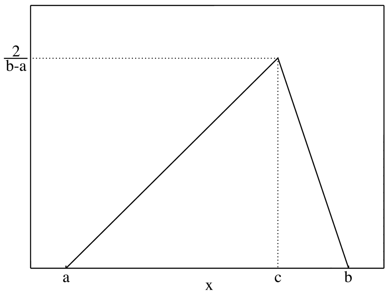
To add more information to the estimate, we assign each item a low, likely and high cost. The low cost ($a$) is rarely achieved and is your ‘bargain-basement’ price. The likely cost ($c$) is what you would typically use in your estimate. Finally, the high cost ($b$) is what you will pay when everything you can think of goes wrong. Statistically, each cost item now has a triangular probability distribution, visualised below.

Our cost estimate would now look something like this:
| Item | Low | Medium | High |
|---|---|---|---|
| Materials | 900000 | 909000 | 950000 |
| Excavation | 33000 | 49500 | 50000 |
| Pipe laying | 156000 | 186000 | 200000 |
For each item, we can calculate the average or any other percentile. The average cost of an item is $\frac{a+b+c}{3}$. The expected cost $x$ with likelihood $p$ is defined by the quantiles for each item, given by:
$$x_p = \begin{cases} a + \sqrt{(b-a)(c-a)p} & 0 \leq p \leq p_c \\ b - \sqrt{(b-a)(b-c)(1-p)} & p_c < p \leq 1 \end{cases}$$
Where $p_c$ is the probability of the likely estimate ($c$): $p_c=\frac{c-a}{b-a}$, and $a \leq c$ and $b \geq c$.

While the triangular distribution is the most common method for assessing uncertainty, other distributions are possible; the principles remain the same. Be mindful, however, that most probability distributions range from minus to plus infinity, which is not a realistic assumption for cost estimates.
If your cost estimate contains only one item, you are done, as you can calculate the project cost by plugging in a percentile $p$ into the formulas. The final project cost will be lower than this number at probability $p$. The chosen percentile depends on your risk appetite. A percentile of .95 provides much more confidence that the actual cost will be lower than the budget.
But when the estimate includes multiple items, doing so analytically will be too complex for mere mortals. This situation is where the Monte Carlo technique comes in. The Monte Carlo method simulates reality by calculating thousands of possible outcomes. The result is not a singular number but a distribution of $n$ possible outcomes.
The outcome of a Monte Carlo simulation is a cost estimate for thousands of parallel universes. If you were to undertake the project $n$ times, the distribution of the final cost is expected to resemble the simulation outcome.
Monte Carlo Simulation in R
Several R libraries can calculate triangular distributions. The triangle package provides a set of functions to work with triangular distributions. The rtriangle() function provides a vector of random quantiles for the chosen distribution, as shown below:
  # Monte Carlo Simulation in R
  library(triangle)

  # Triangular distribution
  hist(rtriangle(n = 10000, a = 12000, b = 15000, c = 14000),
       breaks = 100,
       main = "Triangular distribution simulation")
When plotting the histogram of these results, the triangular shape becomes evident, albeit a bit rough around the edges. Notice that a Monte Carlo simulation is only ever an estimate. The higher the number of simulations (in this diagram, 10,000), the higher the resolution of the result. To test this proposition, change the n parameter in the rtriangle() function.

To add the probability distribution of all your cost items, store all simulations in a matrix with n columns (number of simulations) and j (number of cost items) rows. Then, in the next step, you add all the simulated values and create a histogram or calculate percentiles.
The example below reads a CSV file with the same content as the table above. It then creates a results matrix, runs the simulations and calculates and visualises the results.
The set.seed(1234) function fixes the pseudo-random number generator to always use the same 'random' numbers. This way we always have the same result instead of introducing stochastic noise. If you need true randomness, then use a specialised random generator package that obtains numbers form the random.org website.
  ## Read Data
  estimate <- read.csv("data/cost-estimate.csv")

  ## Simulation settings
  n <- 10000 ## Simulations
  j <- nrow(estimate)
  mc_sims <- matrix(ncol = n,
                    nrow = j)

  ## Simulation
  set.seed(1234)
  for (i in 1:j){
    mc_sims[i,] <- rtriangle(n = n,
                             a = estimate$Low[i],
                             b = estimate$High[i],
                             c = estimate$Medium[i])}

  ## Determine estimates and 95th percentile
  mc_results <- colSums(mc_sims)
  p95 <- quantile(mc_results, 0.95)

  ## Visualise
  hist(mc_results, breaks = 100)
  abline(v = p95, col = "red", lwd = 2)
A Monte Carlo simulation outcome is thus never one number but a vector of numbers from which you can analyse. The example below uses the 95th percentile as the budget figure.
Adding triangular distributions will create a new distribution specific to this project. The mc_results vector holds the estimated possible total cost.
To set a budget figure, you need to nominate a percentile. The 50th percentile has an equal chance of being higher or lower than the actual. You should choose the 95th percentile or whatever percentile matches your risk appetite to have more certainty that a sufficient budget is available.

Monte Carlo cost estimates are not only for projects. You can also undertake these calculations at the program level and assess the level of financial risk you hold within the program.
Monte Carlo cost estimates are a powerful tool for better understanding your project. They are, however, like any modelling, subject to the GiGo principle (Garbage-in-Garbage-out). Therefore, determining the low, likely and high costs will require domain knowledge. While these three estimates have their level of uncertainty, they will provide better insights than relying only on a monolithic amount for contingency.
Probabilistic cost estimates do not guarantee that your project will remain under budget, but they help you achieve this elusive goal.
Share this content


