Spike Detection in Water Treatment Data in the R Language

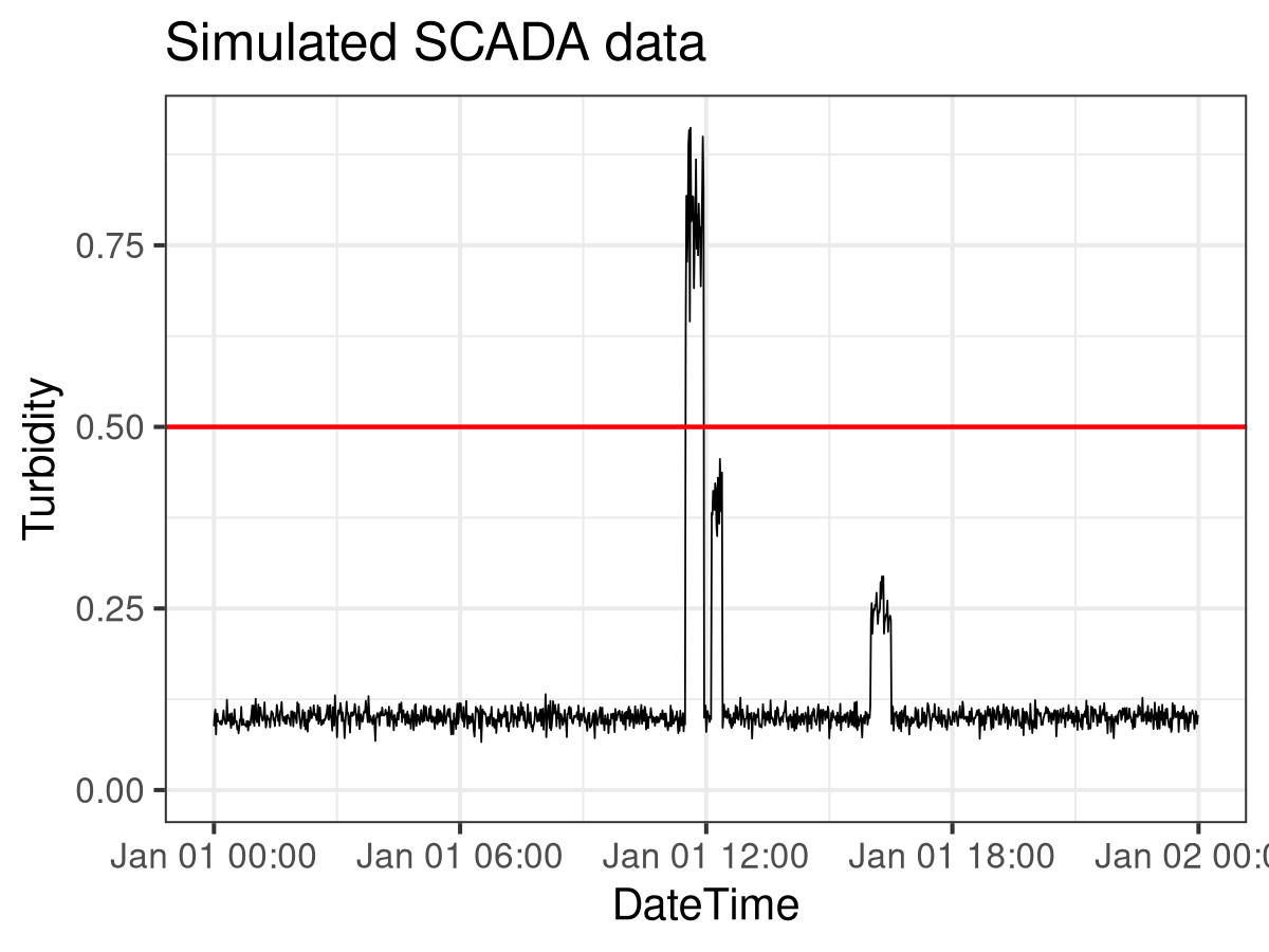
I first created a simulated SCADA feed for turbidity to create a minimum working example. The turbidity data frame contains 24 hours of data. The seq.POSIXt() function creates 24 hours of timestamps at a one-minute spacing. In addition, the rnorm() function creates 1440 turbidity readings with an average of 0.1 NTU and a standard deviation of 0.01 NTU. The image below visualises the simulated data. The next step is to assess this data following the decision rule.

r4h2o

  # Simulate turbidity data

  # set.seed(1234)
  turbidity <- data.frame(timestamp = seq.POSIXt(as.POSIXct("2017-01-01 00:00:00"),
                                                 by = "min",
                                                 length.out = 24 * 60),
                          turbidity = rnorm(n = 24*60,
                                            mean = 0.1,
                                            sd = 0.01))

The second section simulates five spikes in the data. The first line randomly selects a start time for the spike. The second line in the for-loop picks a duration between 10 and 30 minutes. In addition, the third line simulates the spike's value. The mean value of the spike is determined by the rbinom() function to create either a low or a high spike. The remainder of the spike simulation inserts the new data into the turbidity data frame.

  ## Spike detection

  ## Simulate data
  for (i in 1:5) {
    duration <- sample(10:30, 1)
    start_time <- sample(turbidity$timestamp[1:(nrow(turbidity) - duration)], 1)
    value <- rnorm(1, 0.5 * rbinom(1, 1, 0.5) + 0.3, 0.05)
    start_row <- which(turbidity$timestamp == start_time)
    turbidity$turbidity[start_row:(start_row + duration - 1)] <- rnorm(duration, value, value / 10)
  }

  library(ggplot2)

  ggplot(turbidity) + 
    aes(x = timestamp, y = turbidity) + 
    geom_line(size = 0.2) +
    geom_hline(yintercept = 0.5, col = "red", linetype = 2) + 
    ylim(0, max(turbidity$turbidity)) +
    theme_bw(base_size = 10) + 
    ggtitle("Simulated SCADA data")

The image below visualises the simulated data using the mighty ggplot2 package. Only four spikes are visible because two of them overlap. The next step is to assess this data following the decision rule.

The following code searches for all spikes over 0.50 NTU using the runlength function. This function transforms a vector into a vector of values and lengths. For example, the run length of the vector c(1, 1, 2, 2, 2, 3, 3, 3, 3, 5, 5, 6) is:

• lengths: int [1:5] 2 3 4 2 1
• values : num [1:5] 1 2 3 5 6

The value 1 has a length of 1. The value 2 has a length of 3, and so on. The spike detection code computes the run length for turbidity levels greater than 0.5, yielding a boolean vector. The cumsum function calculates the starting point of each spike, which allows us to calculate their duration.

The code produces a data frame containing all spikes above 0.50 NTU and lasting longer than 15 minutes. The spike at 11:29 exceeded 0.50 NTU and lasted 24 minutes. The other three spikes are either lower than 0.50 NTU. The first high spike lasted less than 15 minutes.

  # Spike Detection Function

  spike.detect <- function(timestamp, value, limit, duration) {
    runlength <- rle(value > limit)
    spikes <- data.frame(spike = runlength$values,
                         times = cumsum(runlength$lengths))
    spikes$times <- timestamp[spikes$times]
    spikes$event <- c(0, spikes$times[-1] - spikes$times[-nrow(spikes)])
    spikes <- subset(spikes, spike == TRUE & event > duration)
    return(spikes)
  }

  spike.detect(turbidity$timestamp, turbidity$turbidity, 0.5, 15)

This approach was used to prototype a software package to assess water treatment plant data in accordance with the Health-Based Targets Manual. The finished product has been written in SQL and is available under an free software license.

The book Data Science for Water Utilities discusses anomaly detection in more detail.

As seen on R Bloggers