Simulating Water Consumption to Develop Analysis Tools

For simplicity, this simulation assumes a standard domestic diurnal curve (average daily usage pattern) for indoor water use. Diurnal curves are an essential piece of information in water management. The curve shows water consumption over a day, averaged over a fixed period. The example below is sourced from a journal article. This generic diurnal curve consists of 24 data points based on measured indoor water consumption, shown in the graph below.

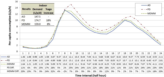
This diurnal curve only includes indoor water consumption and is assumed independent of seasonal variation. This assumption is unrealistic, but the purpose of this simulation is not to accurately model water consumption but to provide a data set to validate the reporting and analyses.

The first code snippet sets the parameters used in this simulation. The unique device identifiers (DevEUI) are simulated as six-digit random numbers. The timestamps vector consists of hourly date-time variables in UTC. For each transmitter, this timestamp is offset by a random time. Each transmitter is also associated with the number of people living in each house. This number is based on a Poisson distribution.

  # Simulate water consumption

  library(tidyverse)

  rm(list = ls())

  # Boundary conditions
  n <- 100 # Number of simulated meters
  d <- 100 # Number of days to simulate
  s <- as.POSIXct("2050-01-01", tz = "UTC") # Start of simulation

  set.seed(1969) # Seed random number generator for reproducibility
  rtu <- sample(1E6:2E6, n, replace = FALSE) # 6-digit id
  offset <- sample(0:3599, n, replace = TRUE) # Unique Random offset for each RTU

  # Number of occupants per connection
  occupants <- rpois(n, 1.5) + 1

  # Visualise
  as_tibble(occupants) %>%
    ggplot(aes(occupants)) + 
    geom_bar(fill = "dodgerblue2", alpha = 0.5) +
    xlab("Occupants") + 
    ylab("Connections") +
    theme_bw(base_size = 10) +   
    labs(title = "Occupants per connection")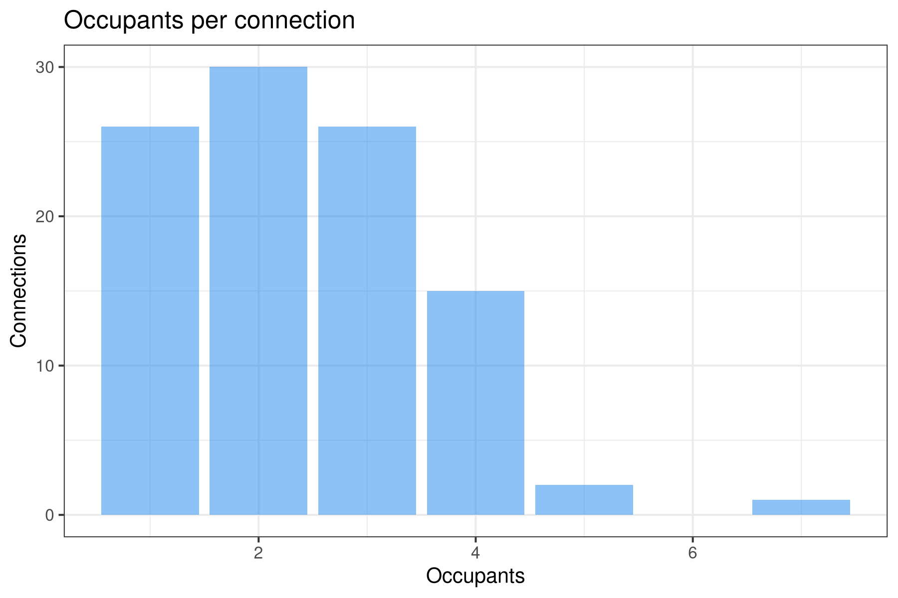

The diurnal curve is based on actual data, including leaks, as the nighttime use shows a consistent flow of about one litre per hour. Therefore, the figures are rounded and reduced by one litre per hour to show a zero flow when people are usually asleep. The curve is also shifted by eleven hours because the raw data is stored in UTC.

  # Diurnal Curve
  diurnal_au <- round(c(1.36, 1.085, 0.98, 1.05, 1.58, 3.87, 9.37, 13.3, 12.1, 10.3, 8.44, 7.04, 6.11, 5.68, 5.58, 6.67, 8.32, 10.0, 9.37, 7.73, 6.59, 5.18, 3.55, 2.11)) - 1

  tdiff <- 11
  diurnal_utc <- c(diurnal_au[(tdiff + 1): 24], diurnal_au[1:tdiff])

This simulation only aims to simulate a realistic data set and not to present an accurate depiction of reality. This simulation could be enhanced by using different diurnal curves for various customer segments, including outdoor watering, temperature dependencies and so on.

A leak is defined by a constant flow through the meter and the idealised diurnal curve. A weighted binomial distribution (θ = 0.1) models approximately one in ten properties with a leak. The size of the leak is derived from a random number between 10 and 50 litres per hour.

The data is stored in a matrix through a loop that cycles through each connection. The DevEUI is repeated over the simulated period (24 times the number of days). The second variable is the timestamp plus the predetermined offset for each RTU.

The meter count is defined by the cumulative sum of the diurnal flow multiplied by the number of occupants. Each point in the diurnal deviates from the model curve by ±10%. Any predetermined leakage is added to each meter read over the whole period of 100 days. The hourly volumes are summed cumulatively to simulate meter reads. The flow is divided by five as each meter revolution indicates five litres.

The following code snippet simulates the digital metering data using the above assumptions and parameters.

  # Leaking properties
  leaks <- rbinom(n, 1, prob = .1) * sample(10:50, n, replace = TRUE)
  data.frame(device_id = rtu, leak = leaks) %>%
    subset(leak > 0)

  # Digital metering data simulation
  meter_reads <- matrix(ncol = 3, nrow = 24 * n * d)
  colnames(meter_reads) <- c("device_id", "timestamp" , "count")

  for (i in 1:n) {
    r <- ((i - 1) * 24 * d + 1):(i * 24 * d)
    meter_reads[r, 1] <- rep(rtu[i], each = (24 * d))
    meter_reads[r, 2] <- seq.POSIXt(s, by = "hour", length.out = 24 * d) + offset[i]
    meter_reads[r, 3] <- round(cumsum((rep(diurnal_utc * occupants[i], d) +
                                       leaks[i]) * runif(24 * d, 0.9, 1.1)) / 5)
  }

  meter_reads <- as_tibble(meter_reads) %>%
    mutate(timestamp = as.POSIXct(timestamp, origin = "1970-01-01", tz = "UTC"))

The data transmission process is not 100% reliable, and the base station will not receive some reads. This simulation identifies reads to be removed from the data through the temporary variable removal. This simulation includes two types of failures:

• Faulty RTUs (2% of RTUs with missing 95% of data)

• Randomly missing data points (1% of data)

    # Set missing indicator
    meter_reads <- mutate(meter_reads, remove = 0)
  
    # Define faulty RTUs (2% of the fleet)
    faulty <- rtu[rbinom(n, 1, prob = 0.02) == 1]
    meter_reads$remove[meter_reads$device_id %in% faulty] <- 
      rbinom(sum(meter_reads$device_id %in% faulty), 1, prob = .5)
  
    # Data loss
    missing <- sample(1:(nrow(meter_reads) - 5), 0.005 * nrow(meter_reads))
    for (m in missing){
      meter_reads[m:(m + sample(1:5, 1)), "remove"] <- 1
    }
  
    # Remove missing reads
    meter_reads <- filter(meter_reads, remove == 0) %>%
      select(-remove)
  
    # Write to disk
    write_csv(meter_reads, "data/meter_reads.csv")
  
    ##Visualise
    filter(meter_reads, device_id %in% sample(faulty, 1)) %>%
      mutate(timestamp = as.POSIXct(format(timestamp,
                                           tz = "Australia/Melbourne"))) %>%
      filter(timestamp >= as.POSIXct("2050-02-06") &
             timestamp <= as.POSIXct("2050-02-08")) %>%
      arrange(device_id, timestamp) %>%
      ggplot(aes(x = timestamp, y = count, colour = factor(device_id))) +
      geom_line() + 
      geom_point()

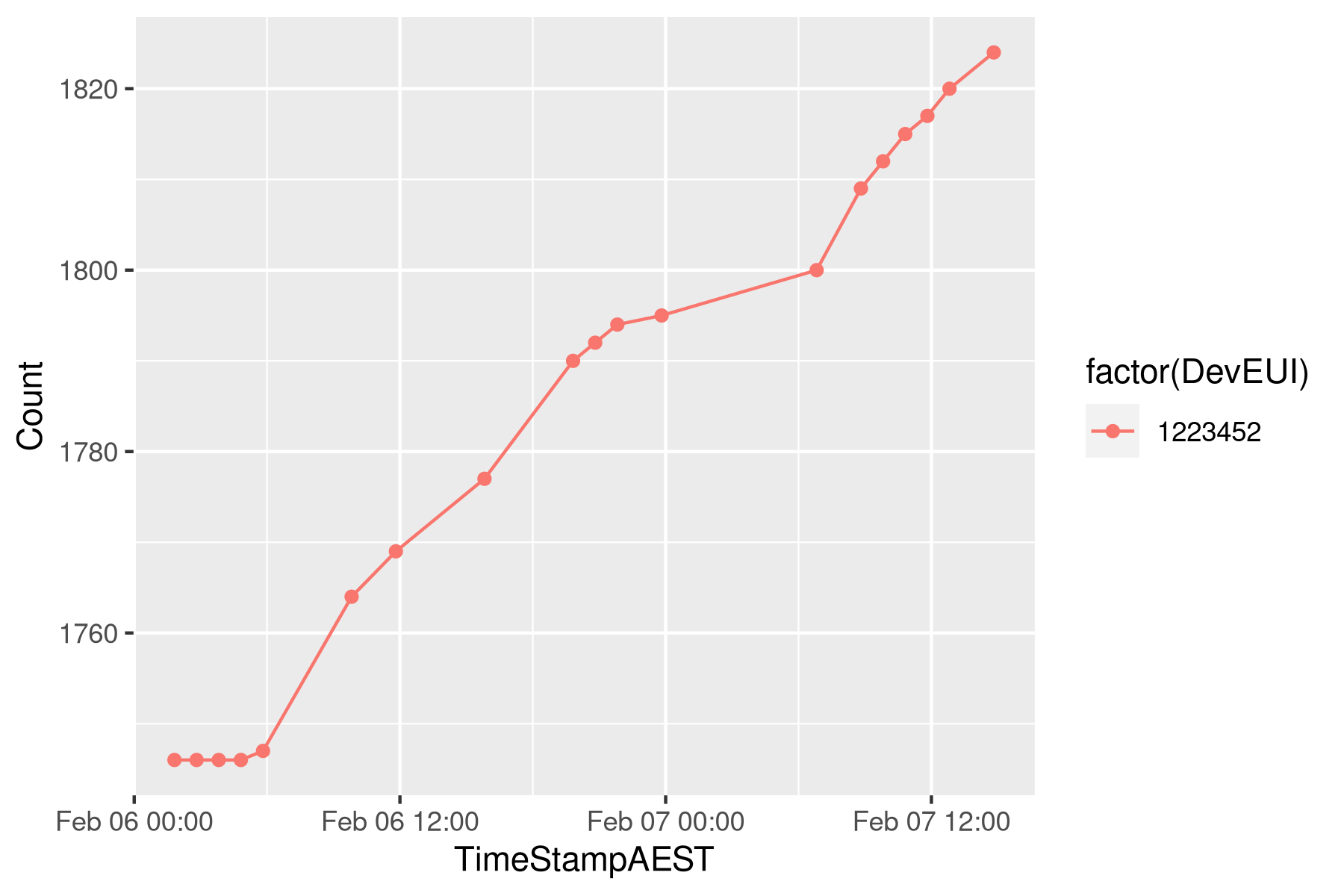
The graph shows an example of the cumulative reads and some missing data points.

Data simulation is a good way to develop your analysis algorithms before you have real data. I have also used this technique while waiting for survey results during my dissertation. When the data finally arrived, I plugged it into the code and finetuned it. R has great capabilities to simulate reality to help you understand the data. The ggplot package provides excellent functionality to visualise water consumption.

In next week's article, I will outline how I used R and the Tidyverse package to develop libraries to analyse digital metering data.

This data was used as a case study in the book Data Science for Water Utilities.

As seen on R Bloggers