Analyse Definitions of Marketing with Rvest and Tidytext

Peter Prevos |
1432 words | 7 minutes
Share this content
I am preparing to facilitate another session of the marketing course for the La Trobe University MBA. The first lecture delves into the definition of marketing. Like most other social phenomena, marketing is tough to define. Definitions of social constructs often rely on the perspective taken by the person or group writing the definition. As such, definitions also change over time. While a few decades ago, definitions of marketing revolved around sales and advertising, contemporary definitions are more holistic and reference creating value.
Heidi Cohen wrote a blog post where she collated 72 definitions of marketing. So rather than arguing over which definition is the best, why not use all definitions simultaneously? This article attempts to define a new definition of marketing, using a data science approach. We can use the R language to scrape the 72 definitions from Heidi's website and attempt text analysis to extract the essence of marketing from this data set.
I have mentioned in a previous post about qualitative data science that automated text analysis is not always a useful method to extract meaning from a text. I decided to delve a little deeper into automated text analysis to see if we find out anything useful about marketing using the rvest and tidytext packages.
Scraping Definitions of Marketing with Rvest
Web scraping is a technique to download data from websites where this data is not available as a clean data source. Web scraping starts with downloading the HTML code from the website and the filtering the wanted text from this file. The rvest package simplifies this process.
The code for this article uses a pipe (%>%) with three rvest commands. The first step is to download the wanted html code from the web using the read_html function. The output of this function is piped to the html_nodes function, which does all the hard work. In this case, the code picks all lines of text that are embedded in an ordered list. You can use the SelectorGadget to target the text you like to scrape. The last scraping step cleans the text by piping the output of the previous commands to the html_text function.
The result of the scraping process is converted to a Tibble, which is a type of data frame used in the Tidyverse. The definition number is added to the data, and the Tibble is converted to the format required by the Tidytext package. The resulting data frame is much longer than the 72 definitions because there are other lists on the page. Unfortunately, I could not find a way to filter only the 72 definitions.
  library(tidyverse)
  library(rvest)
  library(tidytext)
  library(wordcloud)
  library(RColorBrewer)
  lm_palette <- c("#f7881f", "#55ace1",  "#5f6c36")

  ## Scrape definitions from website
  definitions <- read_html("https://heidicohen.com/marketing-definition/") %>%
      html_nodes("ol li") %>%
      html_text() %>%
      as_tibble() %>%
      mutate(No = 1:nrow(.)) %>%
      select(No, Definition = value)
Tidying the Text
The Tidytext package extends the tidy data philosophy to a text. In this approach to text analysis, a corpus consists of a data frame where each word is a separate item. The code snippet below takes the first 72 rows, and the unnest_tokens function extracts each word from the 72 definitions. This function can also extract ngrams and other word groups from the text. The Tidytext package is an extremely versatile piece of software which goes far beyond the scope of this article. Julia Silge and David Robinson have written a book about text mining using this package, which provides a very clear introduction to the craft of analysing text.
The last section of the pipe removes the trailing "s" from each word to convert plurals into single words. The mutate function in the Tidyverse creates or recreates a new variable in a data frame.
  ## bag of words
  def_words <- definitions[1:72, ] %>%
      unnest_tokens(word, Definition) %>%
      mutate(word = gsub("s$", "", word))
This section creates a data frame with two variables. The No variable indicates the definition number (1–72) and the word variable is a word within the definition. The order of the words is preserved in the row name. To check the data frame you can run unique(def_words$No[which(def_words$word = "marketing")])=. This line finds all definition numbers with the word "marketing", wich results, as expected, in the number 1 to 72.
Using Rvest and Tidytext to define marketing
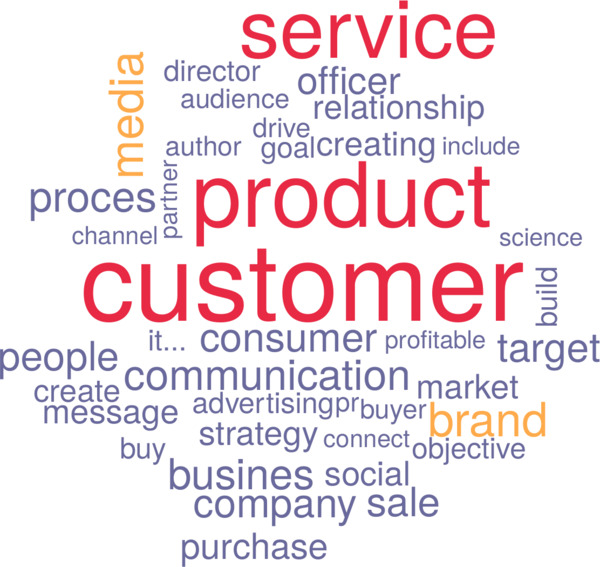
We can now proceed to analyse the definitions scraped from the website with Rvest and cleaned with Tidytext. The first step is to create a word cloud, which is a popular way to visualise word frequencies. This code creates a data frame for each unique word, excluding the word marketing itself, and uses the wordcloud package to visualise the fifty most common words.
  word_freq <- def_words %>%
      anti_join(stop_words) %>%
      count(word) %>%
      filter(!(word %in%
               c("marketing", "vice", "president", "chief", "executive", "’")))

  pdf("marketingcloud.pdf")
  word_freq %>%
      with(wordcloud(word, n, max.words = 50, rot.per = .5,
                     colors = rev(lm_palette)))
  dev.off()
While a word cloud is indeed a pretty way to visualise the bag of words in a text, it is not the most useful way to get the reader to understand the data. The words are jumbled, and the reader needs to search for meaning. A better way to visualise word frequencies is a bar chart. This code takes the data frame created in the previous snippet, determines the top ten occurring words. The mutate statement reorders to factor levels so that the words are plotted in order.
    word_freq %>%
        top_n(10) %>%
        mutate(word = reorder(word, n)) %>%
        ggplot(aes(word, n)) + geom_col(fill = lm_palette[2]) +
        coord_flip() +
        theme(text = element_text(size = 15))
    ggsave("marketing-words.png", width = 6, height = 6)
A first look at the word cloud and bar chart suggests that marketing is about customers and products and services. Marketing is a process that includes branding and communication. This definition is simplistic but functional.
Topic Modeling using Tidytext
Word frequencies are a weak method to analyse text because it interprets each word as a solitary unit. Topic modelling is a more advanced method that examines the relationships between words, i.e. the distance between them. The first step is to create a Document-Term Matrix, which is a matrix that indicates how often a word appears in a text. As each of the 72 texts are very short, I decided to treat the collection of definitions as one text about marketing. The cast_dtm() function converts the data frame to a Document-Term Matrix.
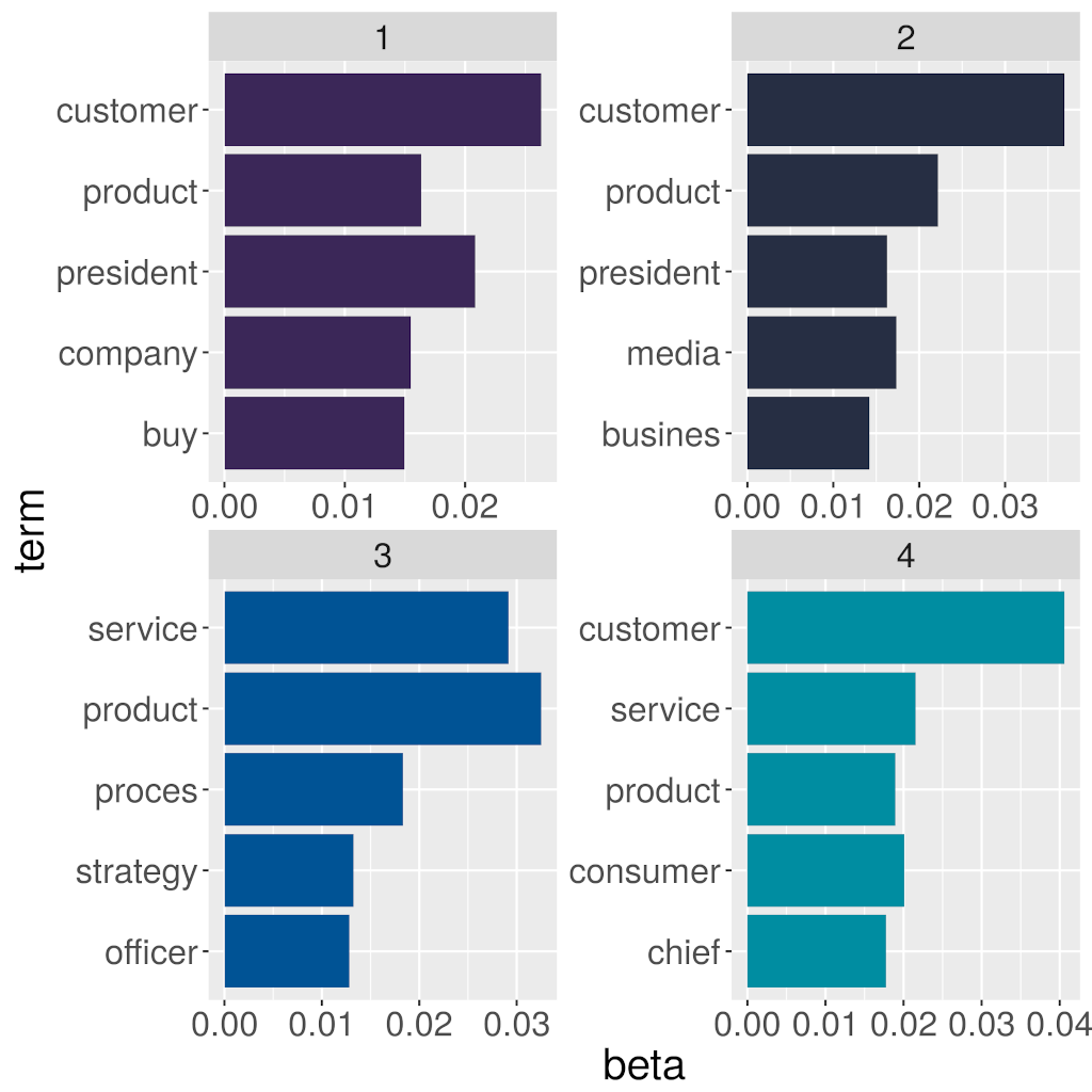
The following pipe determines the top words in the topics. Just like k-means clustering, the analyst needs to choose the number of topics before analysing the text. In this case, I have opted for four topics. The code determines the contribution of each word to the four topics and selects the five most common words in each topic. The faceted bar chart shows each of the words in the four topics.
  ## Topic modeling
  library(topicmodels)

  marketing_dtm <- word_freq %>%
      mutate(doc = 1) %>%
      cast_dtm(doc, word, n)

  marketing_lda <- LDA(marketing_dtm, k = 4) %>%
      tidy(matrix = "beta") %>%
      group_by(topic) %>%
      top_n(5, beta) %>%
      ungroup() %>%
      arrange(topic, -beta)

  marketing_lda %>%
      mutate(term = reorder(term, beta)) %>%
      ggplot(aes(term, beta, fill = factor(topic))) +
      geom_col(show.legend = FALSE) +
         facet_wrap(~topic, scales = "free") +
         coord_flip() +
         theme(text = element_text(size = 20))
This example also does not tell me much more about what marketing is, other than giving a slightly more sophisticated version of the word frequency charts. This chart shows me that marketing is about customers that enjoy a service and a product. Perhaps the original definitions are not distinctive enough to be separated from each other.
This article is only a weak summary of the great work by Julia Silge who co-authored the Tidytext package. The video below provides a comprehensive introduction to topic modelling.
What have we learnt?
This excursion into text analysis using rvest and Tidytext shows that data science can help us to make some sense out of an unread text. If I did not know what this page was about, then perhaps this analysis would enlighten me. This kind of analysis can assist us in wading through to large amounts of text to select the ones we want to read. I am still not convinced that this type of analysis will provide any knowledge beyond what can be obtained from actually reading and engaging with a text.
Although I am a data scientist and want to maximise the use of code in analysing data, I am very much in favour of developing human intelligence before we worry about the artificial kind.
Share this content


