Descriptive Statistics in Water Quality

Peter Prevos |
750 words | 4 minutes
Share this content
The first step in telling data stories is summarising the available data. Descriptive statistics are tools that use a single number to describe a distribution. Analysts calculate averages, medians, percentiles and other statistical summaries to represent a data set's tendency, spread, positions and shape. Statisticians have defined five types of descriptive statistics: frequency, central tendency, position, dispersion and shape. This chapter of Data Science for Water Utilities shows how to calculate descriptive statistics using synthetic water quality data from an imaginary city. The learning objectives for this chapter are:
- Summarise water quality data using various descriptive statistics
- Evaluate compliance of water quality data with relevant regulations.
- Perform grouped data analysis

Data Science for Water Utilities
Data Science for Water Utilities published by CRC Press is an applied, practical guide that shows water professionals how to use data science to solve urban water management problems using the R language for statistical computing.
The data and code used in this chapter are available on GitHub:
Descriptive Statistics
We have already seen measures of frequency in Chapter 3, which count the number of times each observation occurs in a data sample. The remaining four descriptive statistics are:
- Central tendency summarises a distribution with a single number
- Position describes how an observation relates to the others
- Dispersion describes how far the data deviates from the central tendency
- Shape summarises the shape of a distribution
Measure of Central Tendency
A central tendency summarises a distribution with a single number, such as the mean, median or mode.
R has the mean() and median() functions, but no basic function to calculate the mode is available but can easily be added. Water quality data tends to be heavily skewed, so care needs to be taken when using the mean to describe a sample of water quality samples.

Measures of Position
A measure of position is a number’s relative position within the sample. Examples of measures of position are quartiles, deciles, and percentiles, generically known as a quantile. A percentile is a quantile multiplied by 100. Percentiles are a standard method to describe water quality data. For example, if we state that the 95th percentile of turbidity was 4 NTU, 95% of results were lower than or equal to 4 NTU, allowing the occasional spike. An earlier article on the website describes how R undertakes percentile calculations in more detail.
Measures of Dispersion
Dispersion is the extent to which the measurements are spread. Several measures are available, such as the range and Inter-Quartile-Range, variance and standard deviation. The base R package has built-in functions for each of these measures. Please note that R uses Bessel’s Correction to calculate variances to correct the bias in the estimated population variance.
Measures of Shape
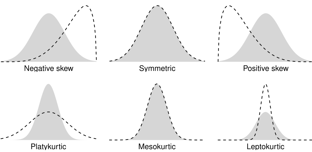
Lastly, we also need to know something about the shape of the distribution. The skewness of a distribution measure the eccentricity of the distribution curve. The kurtosis measures the ‘fatness’ of the tails of the distribution. A high skewness and kurtosis are, therefore, a sign of outliers in the data.

The moments and e1071 packages provide functions to calculate skewness and kurtosis. These packages use slightly different approaches, so the results can differ. Refer to the book or the package documentation for details.
Grouping Data
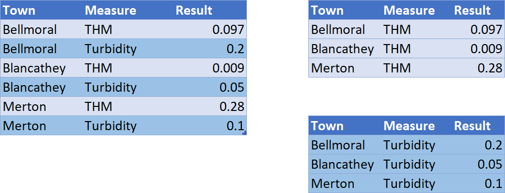
Most data sets contain observations from various groups of data. In this case, we can analyse data by analyte, suburb or sample point. The group_by() function in the dplyr package creates a grouped data frame which means you can calculate descriptive statistics by group. The example below shows a subset of the water quality data, and the two tables on the right are grouped by measure (analyte). The summarise function is the workhorse that lets us analyse the data frame for each group.

Descriptive Statistics in R Screencast
Chapter four of Data Science for Water Utilities explains descriptive statistics and how to calculate them in R in more detail. This screencast below reviews the code for this chapter.
The data and code used in this chapter are available on GitHub:
Additional Resources
To help you remember the various functions discussed in the first five chapters of the book, a cheat sheet is available.
Other Chapters
Previous Chapter: Loading and Exploring Data
Next Chapter: Visualing Water Quality Data with ggplot2.
Feel free to contact me if you have any comments, suggestions or questions about this book.
Share this content


